I had a show and tell session with the folks at PIL a few days ago where I showed off how JPEG image compression actually works, by making a python notebook that uses NumPy for implementing the steps. However, I skimped over understanding one crucial part of JPEG that makes it all work: 2D Discrete Cosine Transform (DCT).
You could access the notebooks explaining JPEG and a few other experiments I tried out here
What is Discrete Cosine Transform (DCT)?
Cosine Transform is one of many transforms used on discrete signals to change their representation from the spatial domain (or time domain) into the frequency domain as a sum of cosine waves.
There are multiple variants of DCT (numbered Types I through VIII), differing in how they assume the boundary conditions and symmetric periodic extensions. However, in this post, I'm only interested in two types, DCT-I and DCT-II (the type used in JPEG):
- DCT-I: Assumes even symmetry around the exact boundary sample points (without repeating the endpoints).
- DCT-II: Shifts the sampling grid by half a sample width ($x + 1/2$) and mirrors boundaries symmetrically with repetition. This offers near-optimal energy compaction for natural signals and minimizes boundary discontinuities.
Because of this property, DCT-II is universally known as "the DCT" and is the standard variant used in compression algorithms like JPEG and MP3.
The 1D DCT (Type-II) is defined as: $$F(u) = \sum_{x=0}^{N-1} f(x) \cos\left(\frac{(2x+1)u\pi}{2N}\right)$$
where:
- $f(x)$ is the input value at index $x$
- $N$ is the length of the 1D sequence
- $u$ is the discrete frequency index ($0 \le u < N$)
In 2D signal processing (like image compression), the 1D DCT is applied across both dimensions (rows and columns). This is vastly helpful because most natural images contain mostly low-frequency information (smooth gradients and uniform regions) and very little high-frequency information (sharp edges, noise).
So how does 2D DCT work?
An image is a two-dimensional grid of pixels. To transform a 2D block of pixels into frequency space, we apply the 2D DCT.
In JPEG, the image is first split into color channels (Luminance $Y$, and Chrominance $Cb, Cr$), and each channel is divided into $8\times8$ pixel blocks ($M = 8, N = 8$).
The 2D DCT-II formula for an $M \times N$ block is:
$$ F(u,v) = \frac{2}{\sqrt{MN}} C(u) C(v) \sum_{x=0}^{M-1} \sum_{y=0}^{N-1} f(x,y) \cos\left(\frac{(2x+1)u\pi}{2M}\right) \cos\left(\frac{(2y+1)v\pi}{2N}\right) $$
Where:
- $f(x,y)$ is the pixel intensity (or level-shifted value) at spatial coordinates $(x,y)$
- $M, N$ are the block dimensions ($8\times8$ in JPEG)
- $u, v$ are the horizontal and vertical frequency indices ($0 \le u < M, \; 0 \le v < N$)
- $C(k) = \frac{1}{\sqrt{2}}$ for $k=0$, and $C(k) = 1$ for $k > 0$ (orthogonal scaling factors)
A few interesting facts:
-
The 2D cosine kernel is separable, which means computing a 2D DCT is basically computing a 1D DCT across all rows, followed by a 1D DCT across all columns of the resulting matrix: $$\cos\left(\frac{(2x+1)u\pi}{2M}\right) \cos\left(\frac{(2y+1)v\pi}{2N}\right)$$
-
The top-left coefficient $F(0,0)$ is the DC coefficient representing the average brightness/color across the entire $8\times8$ block (zero frequency). The rest of the coefficients, or AC coefficients, represent increasingly higher-frequency detail, directional edges, and texture variations.
-
Any $8\times8$ patch is decomposed into a weighted sum of 64 fixed basis patterns. Each $F(u,v)$ value acts as the weight (amplitude) for its corresponding pattern:
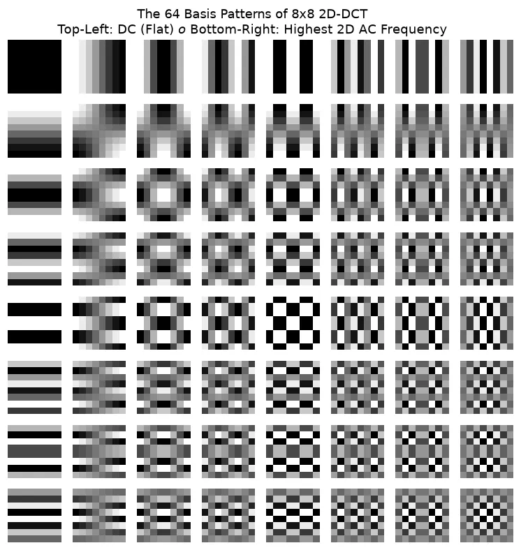
The reason we have 64 fixed basis patterns is that an $8 \times 8$ pixel block contains 64 degrees of freedom (pixels). Because the DCT is a change of basis in a 64-dimensional space, combining 8 horizontal frequencies ($u = 0 \dots 7$) with 8 vertical frequencies ($v = 0 \dots 7$) produces exactly $8 \times 8 = 64$ orthogonal basis patterns needed to reconstruct any arbitrary $8 \times 8$ block.
Because human vision is far less sensitive to fine high-frequency patterns (towards the bottom-right) than smooth low-frequency transitions (towards the top-left), JPEG can aggressively quantize and discard those high-frequency coefficients without noticeable loss in image quality.
The main compression gain comes from the quantisation of this transformed matrix, all while preserving maximum details of the image. Very cool indeed :D